Introduction to grwat R package

Example data

Throughout grwat package documentation a sample dataset spas containing the daily runoff data for Spas-Zagorye gauge on Protva river in Central European plane is used. The dataset is supplemented by meteorological variables (temperature and precipitation) obtained from CIRES-DOE (1880-1949) and ERA5 (1950-2021) data averaged inside gauge’s basin:

library(grwat)
library(dplyr)
library(ggplot2)
library(lubridate)

data(spas)
head(spas)
#> # A tibble: 6 × 4
#>   Date           Q   Temp  Prec
#>   <date>     <dbl>  <dbl> <dbl>
#> 1 1956-01-01  5.18  -6.46 0.453
#> 2 1956-01-02  5.18 -11.4  0.825
#> 3 1956-01-03  5.44 -10.7  0.26 
#> 4 1956-01-04  5.44  -8.05 0.397
#> 5 1956-01-05  5.44 -11.7  0.102
#> 6 1956-01-06  5.58 -20.1  0.032

This 4-column representation is standard for advanced separation discussed below.

Baseflow filtering

For more information on baseflow filtering, read the Baseflow filtering vignette.

grwat implements several methods for baseflow filtering. The get_baseflow() function does the job:

Qbase = gr_baseflow(spas$Q, method = 'lynehollick', a = 0.925, passes = 3)
head(Qbase)
#> [1] 3.698598 3.789843 3.876099 3.958334 4.037031 4.112454

Though get_baseflow() needs just a vector of runoff values, it can be applied in a traditional tidyverse pipeline like follows:

# Calculate baseflow using Jakeman approach
hdata = spas %>% 
  mutate(Qbase = gr_baseflow(Q, method = 'jakeman'))

# Visualize for 2020 year
ggplot(hdata) +
  geom_area(aes(Date, Q), fill = 'steelblue', color = 'black') +
  geom_area(aes(Date, Qbase), fill = 'orangered', color = 'black') +
  scale_x_date(limits = c(ymd(19800101), ymd(19801231)))
#> Warning: Removed 23376 rows containing non-finite values (`stat_align()`).
#> Removed 23376 rows containing non-finite values (`stat_align()`).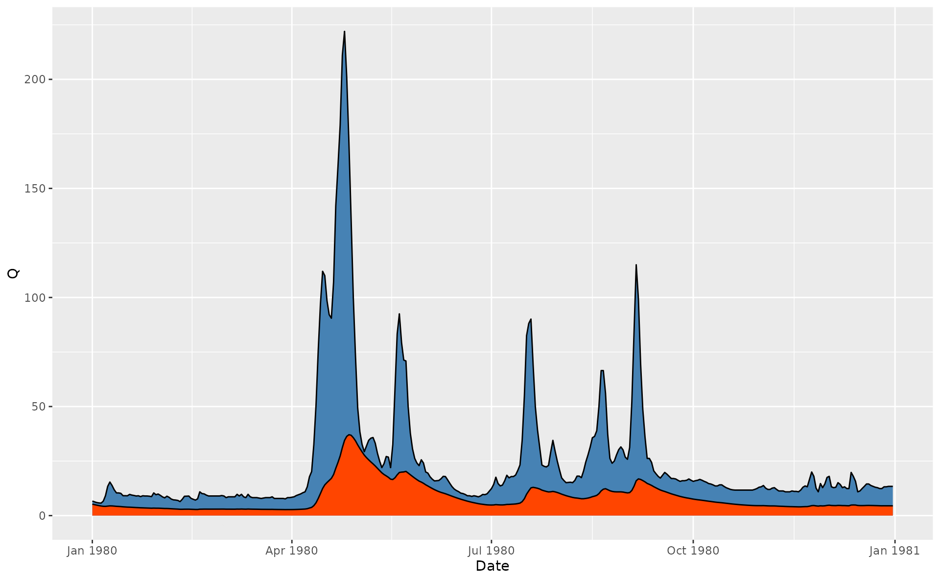

Advanced hydrograph separation

For more information on advanced separation, read the Advanced separation vignette.

Advanced separation by gr_separate() implements the method by (Rets et al. 2022), which involves additional data on temperatures and precipitation to detect and classify flood events into the rain, thaw and spring (seasonal thaw). Between these events \(100\%\) of the runoff is considered to be ground. Inside those events the ground flow is filtered either by one of the baseflow functions, or by Kudelin’s method, which degrades baseflow to \(0\) under the maximum runoff value during the year.

The method is controlled by more than 20 parameters, which can be region-specific. Therefore, to ease the management and distribution of these parameters, they are organized as list, as returned by gr_get_params():

sep = gr_separate(spas, params = gr_get_params(reg = 'center'))
#> grwat: data frame is correct
#> grwat: parameters list and types are OK
head(sep)
#> # A tibble: 6 × 11
#>   Date           Q   Temp  Prec Qbase Quick Qspri Qrain Qthaw Season  Year
#>   <date>     <dbl>  <dbl> <dbl> <dbl> <dbl> <dbl> <dbl> <dbl>  <int> <int>
#> 1 1956-01-01  5.18  -6.46 0.453    NA    NA    NA    NA    NA     NA    NA
#> 2 1956-01-02  5.18 -11.4  0.825    NA    NA    NA    NA    NA     NA    NA
#> 3 1956-01-03  5.44 -10.7  0.26     NA    NA    NA    NA    NA     NA    NA
#> 4 1956-01-04  5.44  -8.05 0.397    NA    NA    NA    NA    NA     NA    NA
#> 5 1956-01-05  5.44 -11.7  0.102    NA    NA    NA    NA    NA     NA    NA
#> 6 1956-01-06  5.58 -20.1  0.032    NA    NA    NA    NA    NA     NA    NA

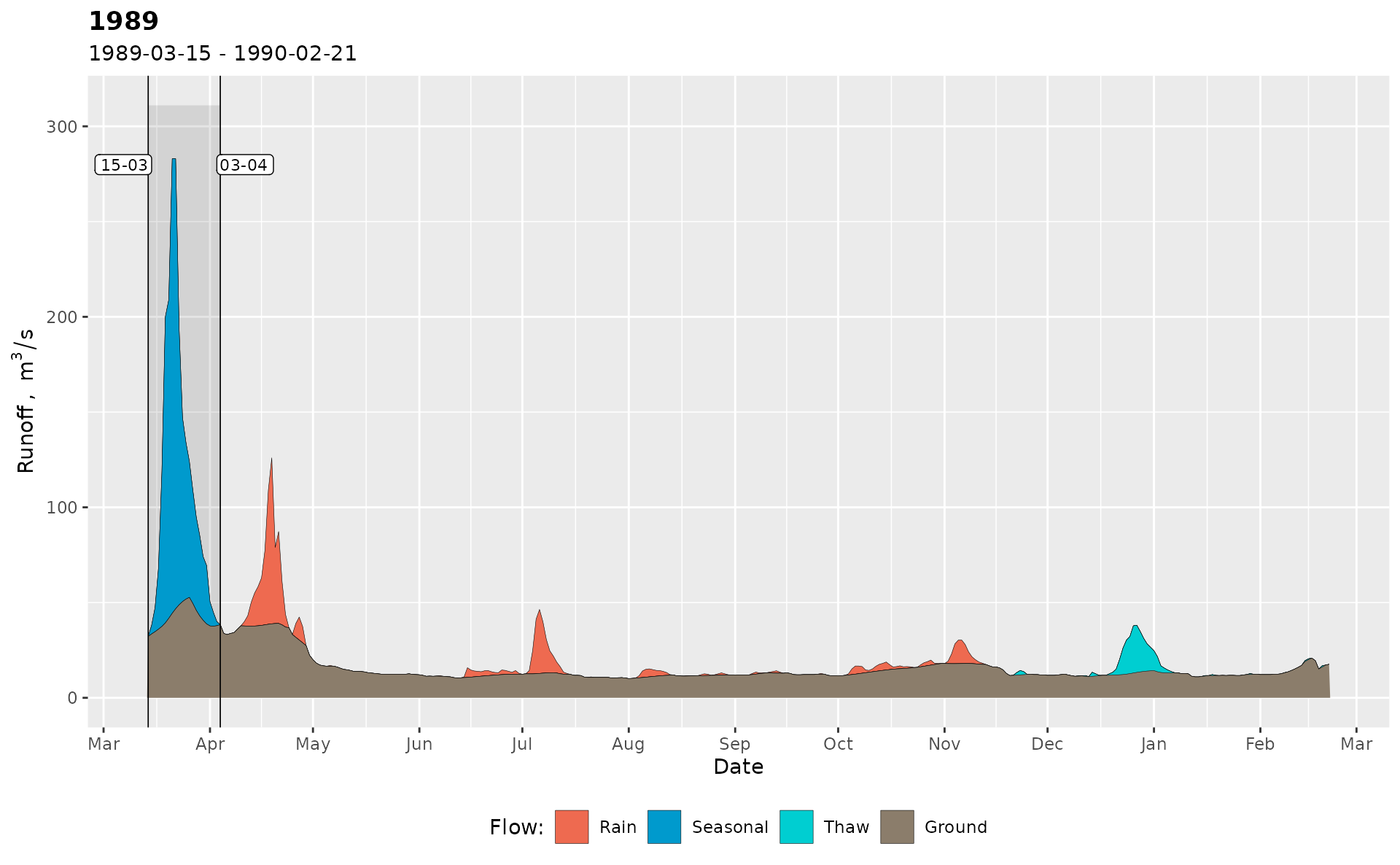
Resulting separation can be visualized by gr_plot_sep() function. In addition to classification of the flow, the function shows the dates of the spring seasonal flood:

gr_plot_sep(sep, years = c(1978, 1989))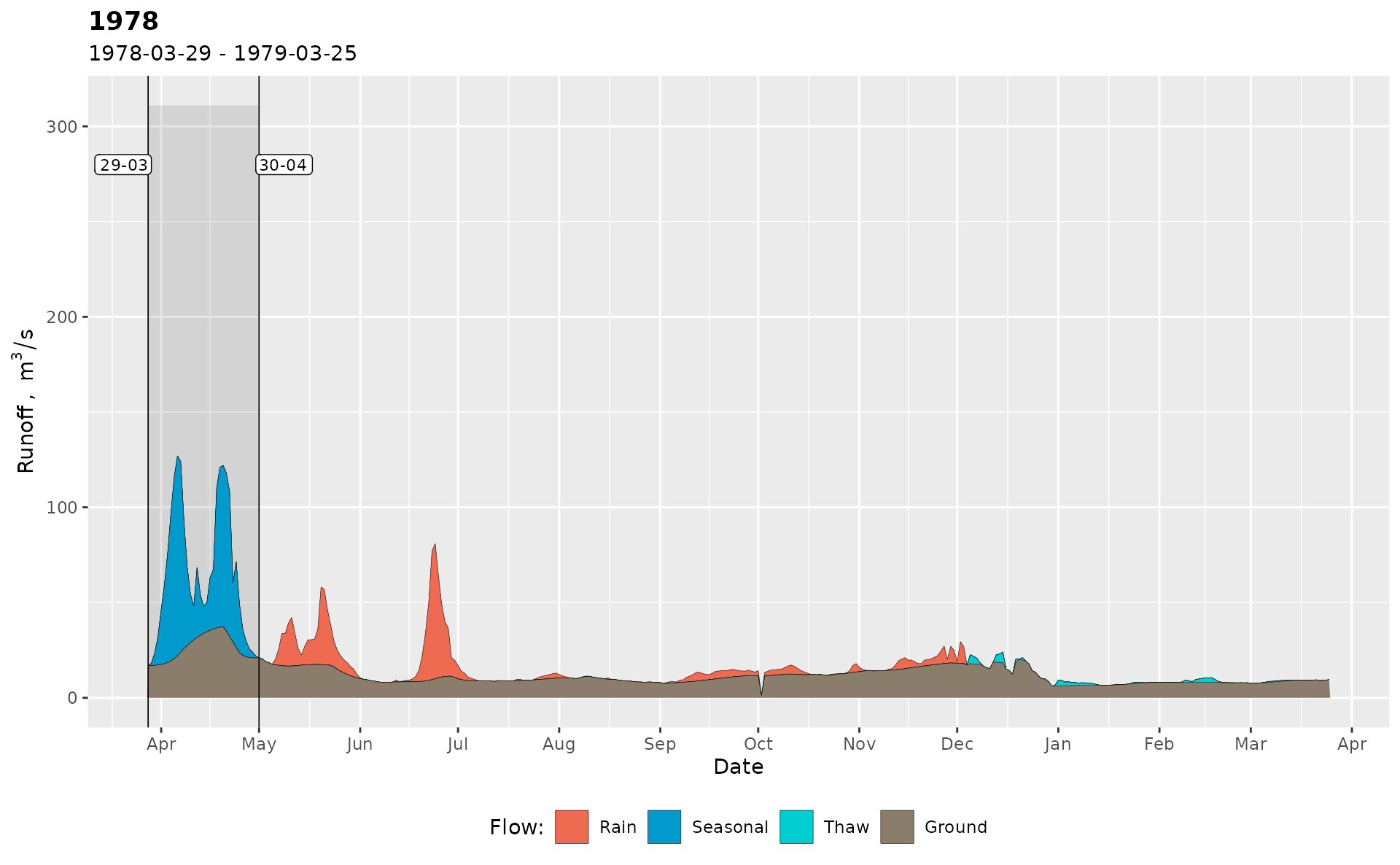

Summaries

For more information on annual variables, read the Summaries vignette.

After hydrograph is separated, its characteristics can be summarized by gr_summarize() into annual variables which characterize the annual runoff, its components (ground, spring, rain and thaw) and low flow periods (summer and winter):

vars = gr_summarize(sep)
head(vars)
#> # A tibble: 6 × 57
#>    Year Year1 Year2 Dspstart   Dspend       Tsp    Qy Qspmax Dspmax      Qygr
#>   <dbl> <dbl> <dbl> <date>     <date>     <int> <dbl>  <dbl> <date>     <dbl>
#> 1  1956  1956  1957 1956-04-08 1956-05-05    27  18.4    467 1956-04-22  8.59
#> 2  1957  1957  1958 1957-03-25 1957-05-04    40  20.2    460 1957-04-08  9.77
#> 3  1958  1958  1959 1958-04-02 1958-05-13    41  27.3    537 1958-04-21 10.2 
#> 4  1959  1959  1960 1959-03-28 1959-04-28    31  27.1    406 1959-04-16 10.9 
#> 5  1960  1960  1961 1960-03-27 1960-04-27    31  29.6    406 1960-04-15 12.3 
#> 6  1961  1961  1962 1961-03-07 1961-05-02    56  18.8    296 1961-04-10 10.8 
#> # ℹ 47 more variables: Qsmin <dbl>, Dsmin <date>, Qwmin <dbl>, Dwmin <date>,
#> #   Q30s <dbl>, D30s1 <date>, D30s2 <date>, Q30w <dbl>, D30w1 <date>,
#> #   D30w2 <date>, Q10s <dbl>, D10s1 <date>, D10s2 <date>, Q10w <dbl>,
#> #   D10w1 <date>, D10w2 <date>, Q5s <dbl>, D5s1 <date>, D5s2 <date>, Q5w <dbl>,
#> #   D5w1 <date>, D5w2 <date>, Wy <dbl>, Wygr <dbl>, Wsp <dbl>, Wspgr <dbl>,
#> #   Wsprngr <dbl>, Wrn <dbl>, Wrngr <dbl>, Wth <dbl>, Wthgr <dbl>, Wgrs <dbl>,
#> #   Ws <dbl>, Wgrw <dbl>, Ww <dbl>, Qrnmax <dbl>, Qthmax <dbl>, …

These characteristics can be plotted by gr_plot_vars():

gr_plot_vars(vars, Qygr)
#> Warning: Removed 1 rows containing non-finite values (`stat_smooth()`).

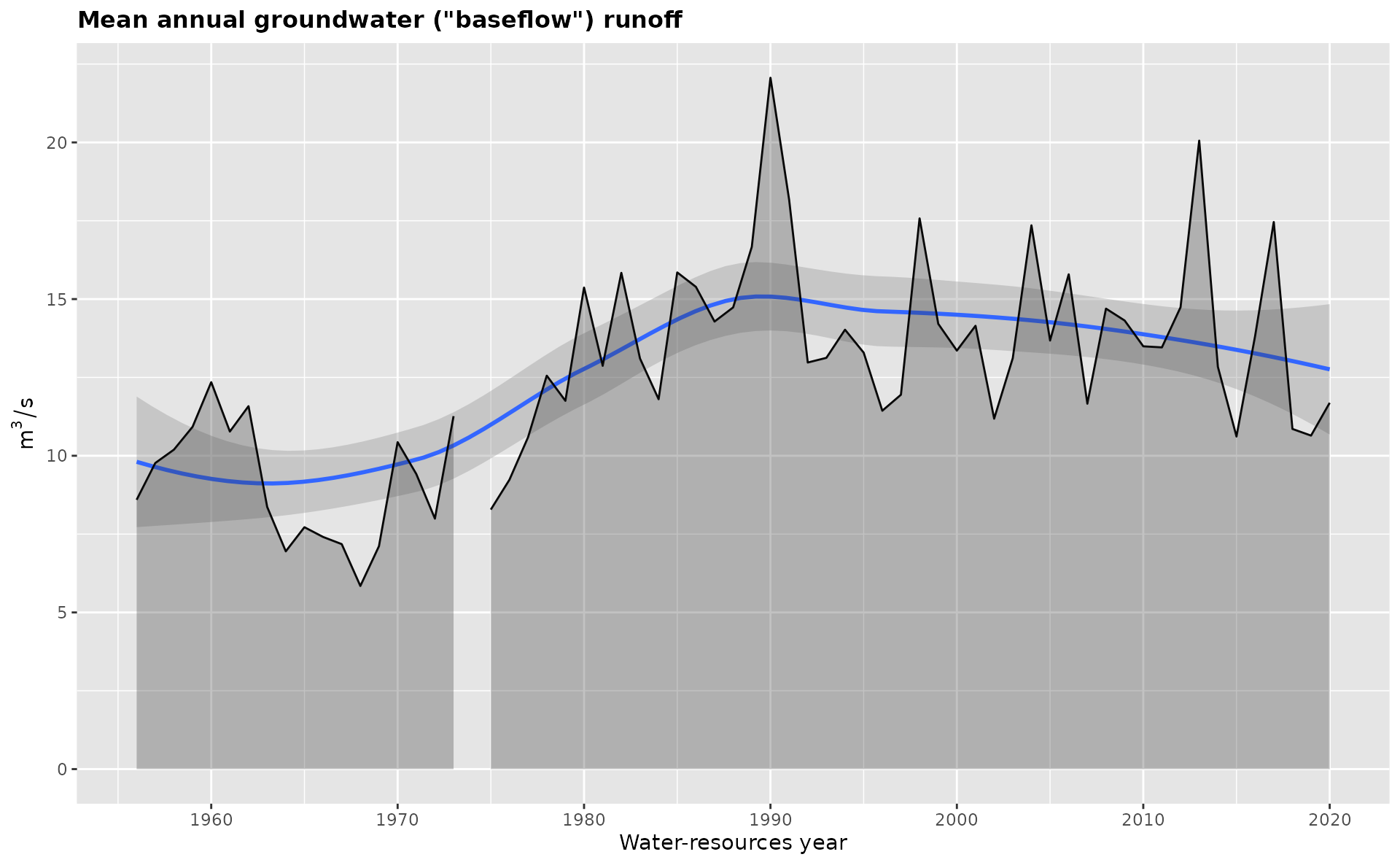
gr_plot_vars(vars, D10w1, Wsprngr, Nthw, Qrnmax, tests = TRUE,
             layout = matrix(1:4, nrow = 2, byrow = TRUE)) 
#> Warning: Removed 1 rows containing non-finite values (`stat_smooth()`).
#> Warning: Removed 1 rows containing missing values (`geom_point()`).
#> Warning: Removed 1 rows containing non-finite values (`stat_smooth()`).
#> Removed 1 rows containing non-finite values (`stat_smooth()`).
#> Warning: Removed 1 rows containing missing values (`geom_rect()`).
#> Warning: Removed 1 rows containing non-finite values (`stat_smooth()`).

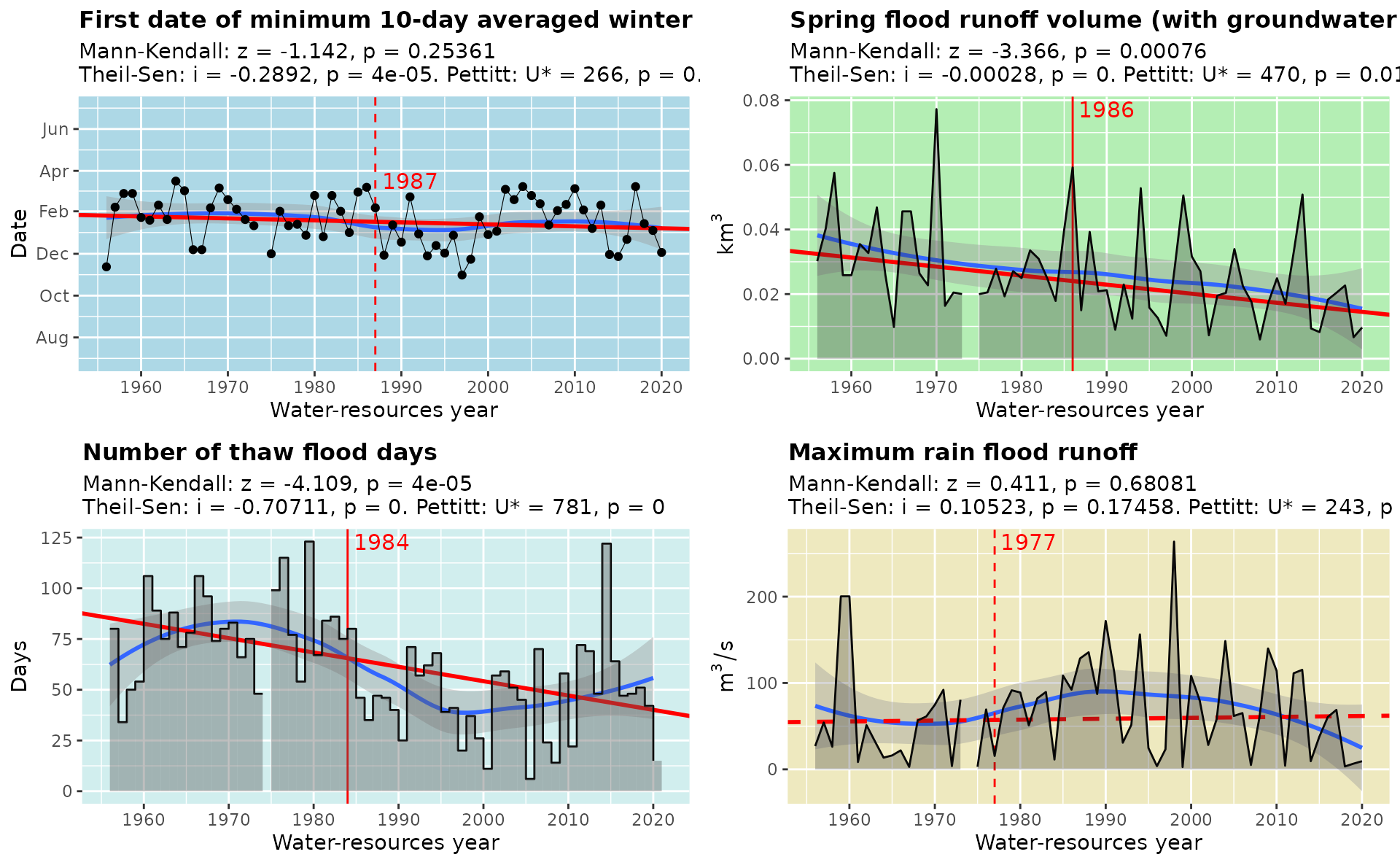
Additional features

grwat contains some useful functions that can facilitate your work with runoff data. In particular:

gr_report() aggregates hydrograph separation and its summaries into one information-rich graphical report that brings everything into one place. Just pass the results of gr_separate() and gr_summarize() into gr_report() function and provide the path to the output HTML file.
gr_get_gaps() and gr_fill_gaps() find and interpolate the periods of missing runoff and meteorological data which may affect the results.
gr_read_rean() and gr_join_rean() add temperature and precipitation to your runoff data from daily reanalysis. This can be useful if you do not have meteorological observations inside the basin. Currently the East European plain is covered.
gr_plot_matrix(), gr_plot_hori() and gr_plot_ridge() empower daily runoff analysis with fascinating graphical techniques which can be used to compare hydrographs for different years: matrix plots, horizon plots and ridgeline plots.
gr_set_locale() translates plots and reports to the specified language (English, Russian and Ukrainian are currently available).
gr_plot_* functions return silently ggplot2 objects or the lists of such objects. This means that they can be modified to your preferences before plotting. Just set print = FALSE and tweak aesthetics as you want or remove some information.

References

Rets, E. P., M. B. Kireeva, T. E. Samsonov, N. N. Ezerova, A. V. Gorbarenko, and N. L. Frolova. 2022. “Algorithm Grwat for Automated Hydrograph Separation by B. I. Kudelin’s Method: Problems and Perspectives.” Water Resources 49 (1): 23–37.